Applying Layers to Quantitative Maps
The primary way of getting data from a layers object is as a Pandas DataFrame. Your quantitative map and mask/anatomical image don’t need to have the same field of view and voxel size, they are resampled to a common space as part of the add_map method. The space parameter of the QLayers class dictates whether any maps added to the object are resampled of the same space as the layers (space=layers) or if the layers are resampled to the native space of the map (space=map). The
advantage of working in layer space is that you can produce a wide DataFrame where each row represents a region of tissue in the image and allows you to directly compare the depth and multiple quantitative parameters however it does involve a resampling operation to the quantitative parameter which may not be desirable (especially for noisy data). Working with space=map only allows you to produce a long DataFrame where each row is a single voxel of each quantitative map. Here we’re going to
work with space=layers and return both formats of DataFrame so you can see the difference. Most analysis is easier with a wide DataFrame so we’ll save that variable for use in subsequent steps. Start by importing the necessary libraries.
[1]:
import matplotlib.pyplot as plt
import nibabel as nib
import numpy as np
import seaborn as sns

from qlayers import QLayers

sns.set()
Now we’re going to import a mask and generate layers with a thickness of 1 mm excluding tissue within 10 mm of the pelvis.
[2]:
mask_img = nib.load('data/kidney_mask.nii.gz')
qlayers = QLayers(mask_img, thickness=1, pelvis_dist=10, space='layers')
r2star_map = nib.load('data/r2star.nii.gz')
t1_map = nib.load('data/t1_registered.nii.gz')
qlayers.add_map(r2star_map, 'r2star')
qlayers.add_map(t1_map, 't1')
Making Mesh
Smoothing Mesh
Distance Calculation: 100%|██████████| 3/3 [00:10<00:00,  3.65s/it]
Pelvis Distance Calculation: 100%|██████████| 3/3 [00:11<00:00,  3.81s/it]
[3]:
qlayers.df_long
[3]:
| depth | layer | measurement | value | |
|---|---|---|---|---|
| 0 | 0.691532 | 1.0 | r2star | 35.173016 |
| 1 | 0.640596 | 1.0 | r2star | 35.546364 |
| 2 | 0.885229 | 1.0 | r2star | 34.576439 |
| 3 | 0.680305 | 1.0 | r2star | 33.275753 |
| 4 | 0.622988 | 1.0 | r2star | 27.070265 |
| ... | ... | ... | ... | ... |
| 25993 | 1.011228 | 2.0 | t1 | 2372.752930 |
| 25994 | 1.099274 | 2.0 | t1 | 1094.152222 |
| 25995 | 0.145987 | 1.0 | t1 | 1351.835815 |
| 25996 | 1.185435 | 2.0 | t1 | 922.929932 |
| 25997 | 0.378006 | 1.0 | t1 | 1491.548584 |
51996 rows × 4 columns
DataFrames
Here is an example of how to retrieve a layers dataframe in long format. Note that every measurement is on a different row of the DataFrame.
[4]:
print('An example of a long DataFrame')
qlayers.get_df('long').sample(n=100)
An example of a long DataFrame
[4]:
| depth | layer | measurement | value | |
|---|---|---|---|---|
| 1452 | 7.921090 | 8.0 | t1 | 1438.690796 |
| 23167 | 3.070961 | 4.0 | r2star | 16.509024 |
| 9873 | 9.106622 | 10.0 | r2star | 19.951300 |
| 15462 | 7.044881 | 8.0 | t1 | 1522.299683 |
| 21780 | 9.554491 | 10.0 | t1 | 1860.597168 |
| ... | ... | ... | ... | ... |
| 5030 | 8.614227 | 9.0 | r2star | -0.000061 |
| 16761 | 11.531033 | 12.0 | t1 | 1811.737183 |
| 17264 | 3.927006 | 4.0 | r2star | -0.000005 |
| 19380 | 10.379864 | 11.0 | r2star | 27.924768 |
| 83 | 0.151749 | 1.0 | t1 | 1996.951416 |
100 rows × 4 columns
And now an example of a wide DataFrame. Here each row represents properties of a single region of tissue i.e. the \(T_1\) and \(R_2^*\) of the same region.
[5]:
df = qlayers.get_df('wide')
# A little bit of data cleaning
df = df.loc[df['r2star'] > 0.1]
df = df.loc[df['t1'] > 0.1]
df = df.loc[df['layer'] > 0]
df = df.dropna()
print('An example of a wide DataFrame')
df.sample(n=100)
An example of a wide DataFrame
[5]:
| depth | layer | r2star | t1 | |
|---|---|---|---|---|
| 18182 | 2.479600 | 3.0 | 49.999969 | 830.443848 |
| 25187 | 7.304027 | 8.0 | 17.250000 | 1491.552002 |
| 981 | 7.609881 | 8.0 | 18.200880 | 1696.885132 |
| 225 | 3.661174 | 4.0 | 16.167454 | 1498.427856 |
| 9813 | 5.483145 | 6.0 | 17.793419 | 1505.549683 |
| ... | ... | ... | ... | ... |
| 9085 | 3.738994 | 4.0 | 16.756792 | 2189.016602 |
| 14667 | 2.410548 | 3.0 | 18.561234 | 648.623413 |
| 4872 | 6.246225 | 7.0 | 20.113871 | 1326.467773 |
| 12614 | 5.033549 | 6.0 | 18.116539 | 1553.667480 |
| 21237 | 14.467604 | 15.0 | 27.227434 | 1818.611694 |
100 rows × 4 columns
Layer Statistics
These large voxel-by-voxel DataFrames can be used to generate statistics for each layer.
[6]:
df[['layer', 'r2star', 't1']].groupby('layer').agg(('mean', 'median', 'std', np.count_nonzero))
[6]:
| r2star | t1 | |||||||
|---|---|---|---|---|---|---|---|---|
| mean | median | std | count_nonzero | mean | median | std | count_nonzero | |
| layer | ||||||||
| 1.0 | 28.777927 | 27.386422 | 10.120994 | 1306 | 1427.316554 | 1432.761292 | 687.366178 | 1306 |
| 2.0 | 24.798214 | 21.119667 | 9.922550 | 1152 | 1514.067368 | 1498.551514 | 521.878771 | 1152 |
| 3.0 | 22.699811 | 18.791880 | 9.507372 | 1117 | 1548.529686 | 1502.680298 | 418.154056 | 1117 |
| 4.0 | 21.311056 | 17.593157 | 8.999270 | 1079 | 1584.577592 | 1504.680908 | 387.597601 | 1079 |
| 5.0 | 20.659930 | 17.642798 | 8.391686 | 1070 | 1555.793643 | 1515.112427 | 245.470044 | 1070 |
| 6.0 | 20.322622 | 17.716091 | 8.013432 | 998 | 1535.698166 | 1518.424866 | 183.277963 | 998 |
| 7.0 | 20.008837 | 17.834057 | 6.875631 | 939 | 1556.361710 | 1526.548950 | 222.644851 | 939 |
| 8.0 | 20.357808 | 18.393726 | 6.256812 | 939 | 1590.342322 | 1545.794434 | 261.664944 | 939 |
| 9.0 | 21.486777 | 18.754271 | 7.210381 | 1249 | 1647.641340 | 1608.914917 | 251.010749 | 1249 |
| 10.0 | 21.896243 | 19.833168 | 6.528540 | 973 | 1668.680325 | 1629.775635 | 242.975416 | 973 |
| 11.0 | 22.848923 | 20.875158 | 6.762447 | 800 | 1699.698935 | 1657.771057 | 270.711344 | 800 |
| 12.0 | 24.367501 | 22.374521 | 7.467851 | 780 | 1724.054959 | 1686.763916 | 314.218625 | 780 |
| 13.0 | 25.761510 | 23.751545 | 8.236693 | 681 | 1768.263152 | 1727.257935 | 334.313298 | 681 |
| 14.0 | 27.090914 | 25.005579 | 8.590587 | 627 | 1816.391434 | 1759.498901 | 373.740812 | 627 |
| 15.0 | 26.376643 | 24.508926 | 8.273556 | 937 | 1794.624822 | 1747.250732 | 358.172194 | 937 |
| 16.0 | 26.683109 | 25.606609 | 7.597819 | 489 | 1911.763796 | 1814.361206 | 469.923051 | 489 |
| 17.0 | 26.739680 | 25.025603 | 8.242154 | 370 | 1903.686099 | 1863.104370 | 428.545985 | 370 |
| 18.0 | 27.080702 | 26.185752 | 8.125888 | 246 | 1885.025251 | 1872.476135 | 404.513906 | 246 |
| 19.0 | 27.964653 | 26.761284 | 8.542669 | 167 | 1854.224052 | 1826.735474 | 416.656298 | 167 |
| 20.0 | 27.312497 | 26.466608 | 7.030809 | 164 | 1822.542544 | 1736.938843 | 416.622615 | 164 |
| 21.0 | 26.563904 | 26.340168 | 7.246280 | 65 | 2048.189515 | 1752.625488 | 643.742097 | 65 |
| 22.0 | 32.333422 | 30.151463 | 11.298019 | 25 | 1842.424917 | 1678.638062 | 394.083905 | 25 |
| 23.0 | 33.817001 | 29.618130 | 9.046841 | 5 | 1972.630908 | 1783.244507 | 534.599383 | 5 |
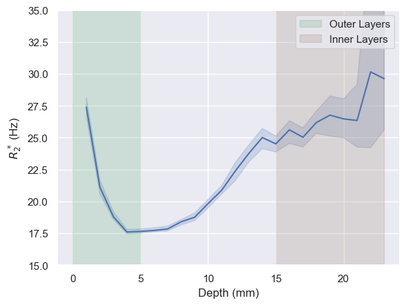
[7]:
fig, ax = plt.subplots()
sns.lineplot(df, x='layer', y='r2star', ax=ax, estimator='median')
ax.set_xlabel('Depth (mm)')
ax.set_ylabel('$R_2^*$ (Hz)')
ax.set_ylim((15, 35))
ax.axvspan(0, 5, alpha=0.2, label='Outer Layers', color='C2')
ax.axvspan(15, 23, alpha=0.2, label='Inner Layers', color='C5')
ax.legend()
[7]:
<matplotlib.legend.Legend at 0x1b6ed946790>